Reading the Lebesgue-number lemma

Read a theorem closely enough to explain when it applies, which choices must work uniformly, and exactly what its conclusion covers.

New to Lean? Read the short notation guide, then start with the same theorem below. You need some familiarity with compact sets, open covers and metric balls.

Already read Lean? Go directly to the source and editor selection. The questions ask you to connect the statement’s scope with its mathematical meaning.

A little Lean notation

Notation used in this example

s : Set α says that s is a set of elements of type α. A family c : ι → Set α assigns a set c i to each index i. Function application is written with a space.

∃ r > 0, P r means there is an r with both 0 < r and P r.
∀ z ∈ s, P z means that every z satisfying z ∈ s satisfies P z.
A ⊆ B means every element of A belongs to B. ⋃ i, c i is the union of all sets in the family.
Braces such as {s : Set α} introduce implicit parameters. Square brackets such as [PseudoMetricSpace α] request a mathematical structure that Lean supplies through its typeclass mechanism.

A pseudometric has the usual metric properties but may assign distance zero to distinct points. No coordinates or dimension are assumed here.

For a broader introduction, use Mathematics in Lean; its Logic chapter explains quantifiers and implications. Theorem Proving in Lean covers Lean’s language in more depth. The lesson below uses only the notation needed for this statement.

Start with the library theorem

Use a trusted project with Lean 4.28.0 and Mathlib revision 8f9d9cff6bd728b17a24e163c9402775d9e6a365, with the import built. This example needs Mathlib, unlike the standard-library files in Lessons 5–7. See Setup for the reader and extension.

Download LebesgueNumber.lean. Its complete source accompanies the recording below.

Open the file in the project and let Lean check it.
Select only lebesgue_number_lemma_of_metric after #check.
Run Definograph: Visualize Selection from the command palette.

The selected theorem constant is a proof term. The main reading presents its proposition type: the statement the theorem proves. #check asks Lean for the constant’s type; it does not construct a radius or a cover index.

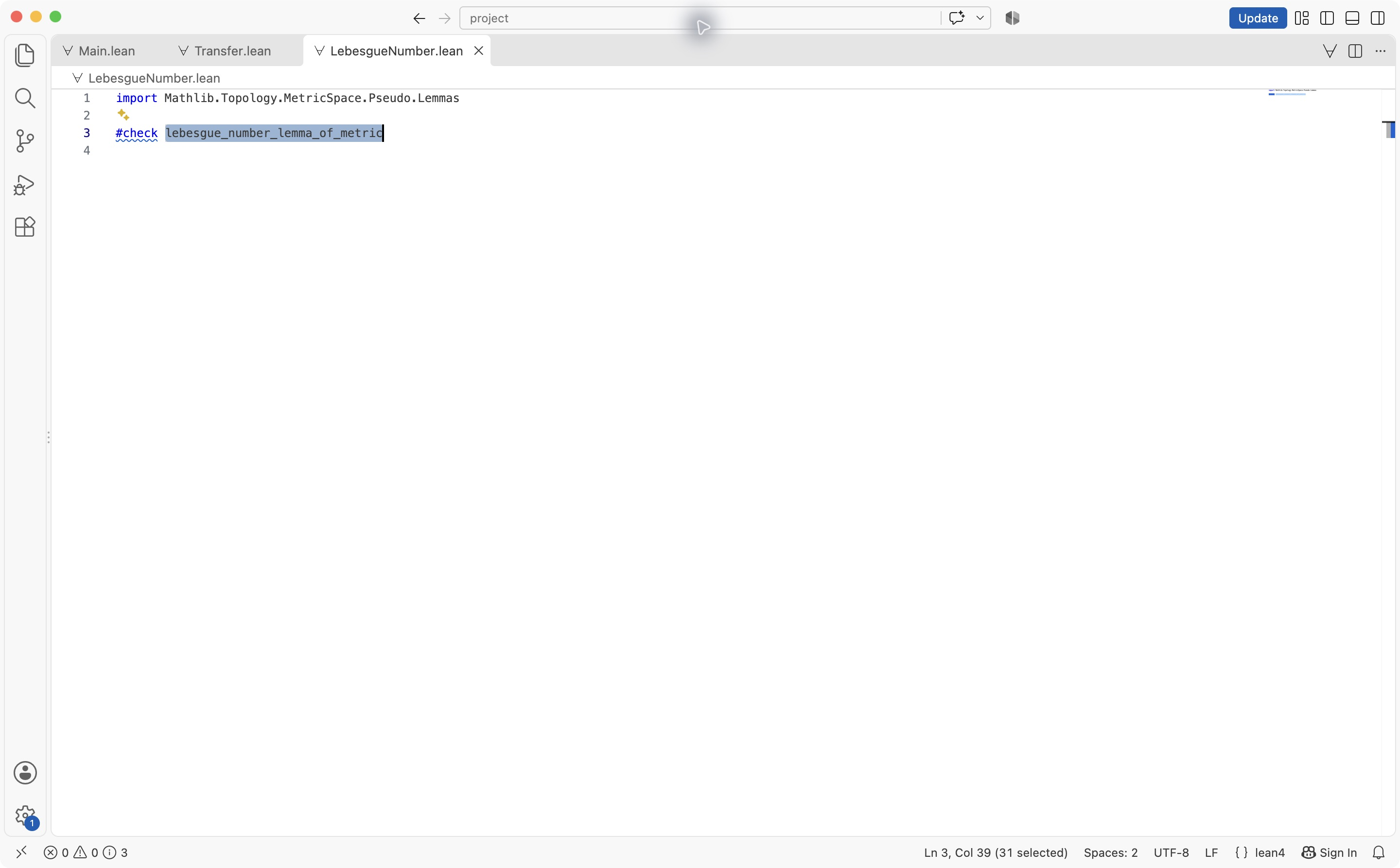
VS Code with LebesgueNumber.lean open and lebesgue_number_lemma_of_metric selected inside the check command. — The theorem name is selected in the editor. Definograph reads the type of this selected proof; the surrounding check command is not itself the theorem’s proof. Open the screenshot on its own.

You can also read the original theorem in Mathlib. Its background consists of a pseudometric space α, a set s, an index sort ι and a family of sets c : ι → Set α. These are the objects and structure in which the theorem is stated.

1. Separate the hypotheses from the conclusion

The theorem has three named hypotheses:

hs : IsCompact s: The set s is compact.
hc₁ : ∀ i, IsOpen (c i): Every member of the family is open.
hc₂ : s ⊆ ⋃ i, c i: The family covers s.

Under these hypotheses, the conclusion is:

∃ δ > 0, ∀ x ∈ s, ∃ i, Metric.ball x δ ⊆ c i

Question. Is knowing that one point lies in one open member enough to apply this theorem? Locate the missing requirements in the whole statement.

Answer: what must be known

No. The theorem requires compactness of s, openness of every family member and coverage of all of s, in the stated pseudometric space. Coverage of one point alone does not provide these hypotheses.

The space, set and family are background data. Do not count them as extra propositional hypotheses alongside hs, hc₁ and hc₂.

2. Read the choices in order

Question. May the radius δ change after choosing x? Must the same index i work for every x?

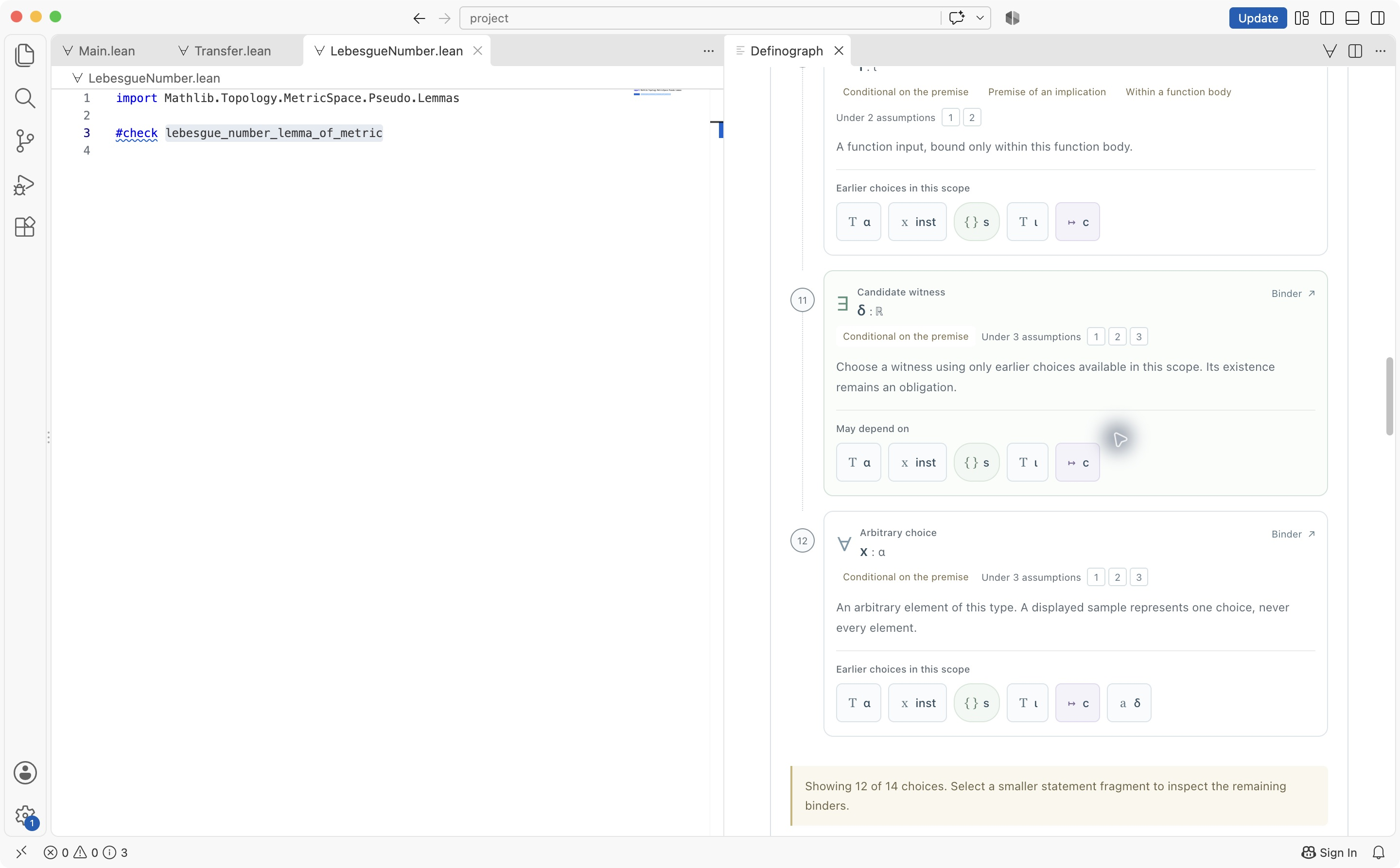
Select Explore a sample, then Choices. The recorded view shows the candidate radius δ before the arbitrary center x; δ appears among the earlier choices available to x. This view displays 12 of the statement’s 14 choices, so the final existential index i is beyond its display limit. Read that choice in the whole statement or the Visual sequence, and keep the conditions in view. A list of choices alone does not show every condition.

The installed Choices view shows candidate radius delta at step 11 before arbitrary center x at step 12, followed by its 12-of-14-choices limit. — The candidate radius δ comes before the center x, and δ appears among the earlier choices available to x. The view explicitly stops after 12 of 14 choices. The later existential index i must be read in the whole statement or Visual sequence; it is not shown here. Open the screenshot on its own.

Answer: one radius, a possibly varying index

A single positive δ is chosen before x and must work for every x ∈ s. Its choice may use the fixed space, set and cover. It cannot be chosen afresh for each later point.

The index i comes after x and its membership condition. It may vary with x; the theorem neither requires variation nor supplies a procedure for choosing the index.

δ > 0 is part of what the conclusion guarantees about its radius. It is joined to the remaining conclusion under ∃ δ, rather than being an extra hypothesis required before applying the theorem.

3. Read the whole-ball requirement

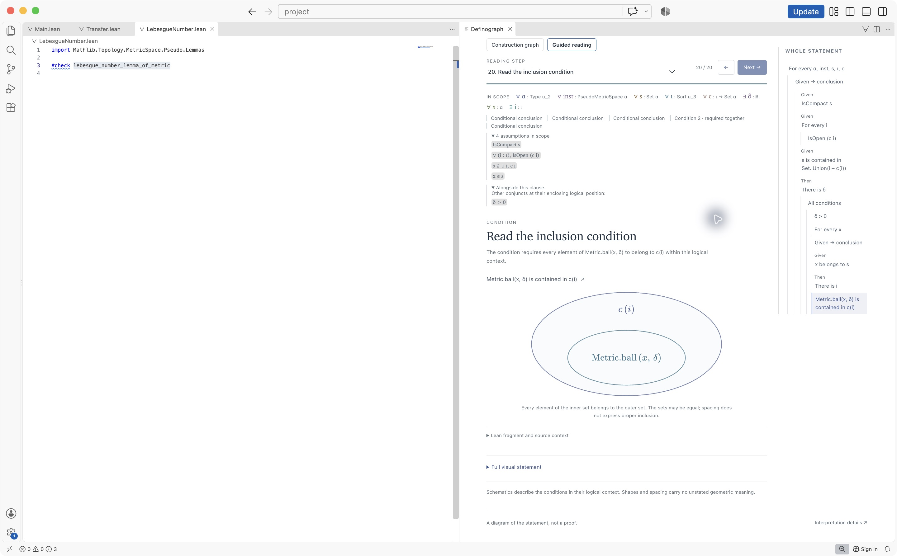
Select Visual sequence, then use Choose reading step to select 20. Read the inclusion condition. Read Metric.ball x δ ⊆ c i with its enclosing scope.

Open 4 assumptions in scope: the theorem’s three hypotheses and the local condition x ∈ s. Open Alongside this clause to retain δ > 0 at its position in the conclusion.

Question. Does the conclusion cover only the center x, only the part of the ball inside s, or the whole ball?

The installed Visual sequence at the inclusion clause, with the four assumptions, positive radius and whole-ball containment. — The inclusion clause requires the whole ball Metric.ball x δ to lie inside c i. Its scope retains the theorem’s three hypotheses and x ∈ s; the positive-radius condition remains alongside the clause. The diagram states a containment requirement and supplies no numerical witness. Open the screenshot on its own.

Answer: which points are covered

Every point of the whole ball belongs to c i, for the index chosen for this center. Only the center x is restricted to s. The theorem does not say that the ball is contained in s.

Replacing the conclusion by x ∈ c i would lose the neighborhood guarantee. Replacing the ball by its intersection with s would also weaken what is stated.

Inspect the ball’s definition

Keep the inclusion clause selected while inspecting the expression Metric.ball x δ:

Select Inspect a definition in this statement.
Enter Metric.ball in Find an application. Applications come from the whole selected statement, so check the occurrence’s arguments and scope. Choose the occurrence with center x and radius δ using Inspect this occurrence →.
In Keep the clause in view, check that Original clause still shows Metric.ball x δ ⊆ c i. Wait for the inspection to complete, then read its result and check outcomes.

The installed definition workspace keeps the original inclusion clause visible and presents the scoped result of inspecting Metric.ball, with three accepted checks. — Inspecting the selected Metric.ball application exposes {y | dist y x < δ} while keeping the original clause in view. The result’s context, component and definition-head conversion are accepted. These checks concern this exposure in its scope; they do not prove the inclusion clause. Notation can hide implicit arguments, available with the exact result and scope. Open the screenshot on its own.

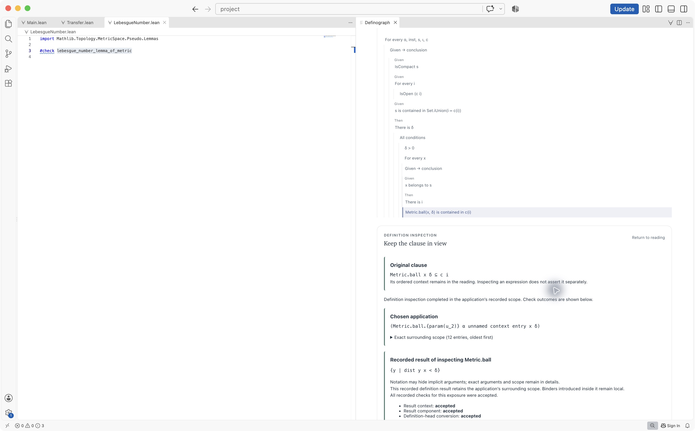
The recorded result of inspecting Metric.ball is:

{y | dist y x < δ}

Notation may hide implicit arguments. Use Exact result and surrounding scope for the exact arguments and scope. The result retains the chosen application’s surrounding scope; the variable y is local to the set description, not a replacement for the center x.

In this recording, Result context, Result component and Definition-head conversion are all marked accepted. These checks concern this definition exposure in its scope; they do not prove the containment clause.

The bound is strict. Combining the definition with the containment clause says that every y satisfying dist y x < δ belongs to the same c i. The pinned library definition of Metric.ball provides a source reference.

4. Put the conclusion back together

Select Return to reading. The definition workspace closes and focus returns to Choose reading step, still on 20. Read the inclusion condition. Check the center, radius and cover member against the original statement, with the four assumptions and δ > 0 still in view.

Question. Explain the conclusion in one sentence, including what is fixed and what may vary.

The installed reader after Return to reading, with the inclusion condition still selected and its scope retained. — Return to reading closes the definition workspace and restores the inclusion clause. The center, common radius and cover member can again be read with the assumptions and positivity condition. The recorded action restores the reading-step control’s focus. Open the screenshot on its own.

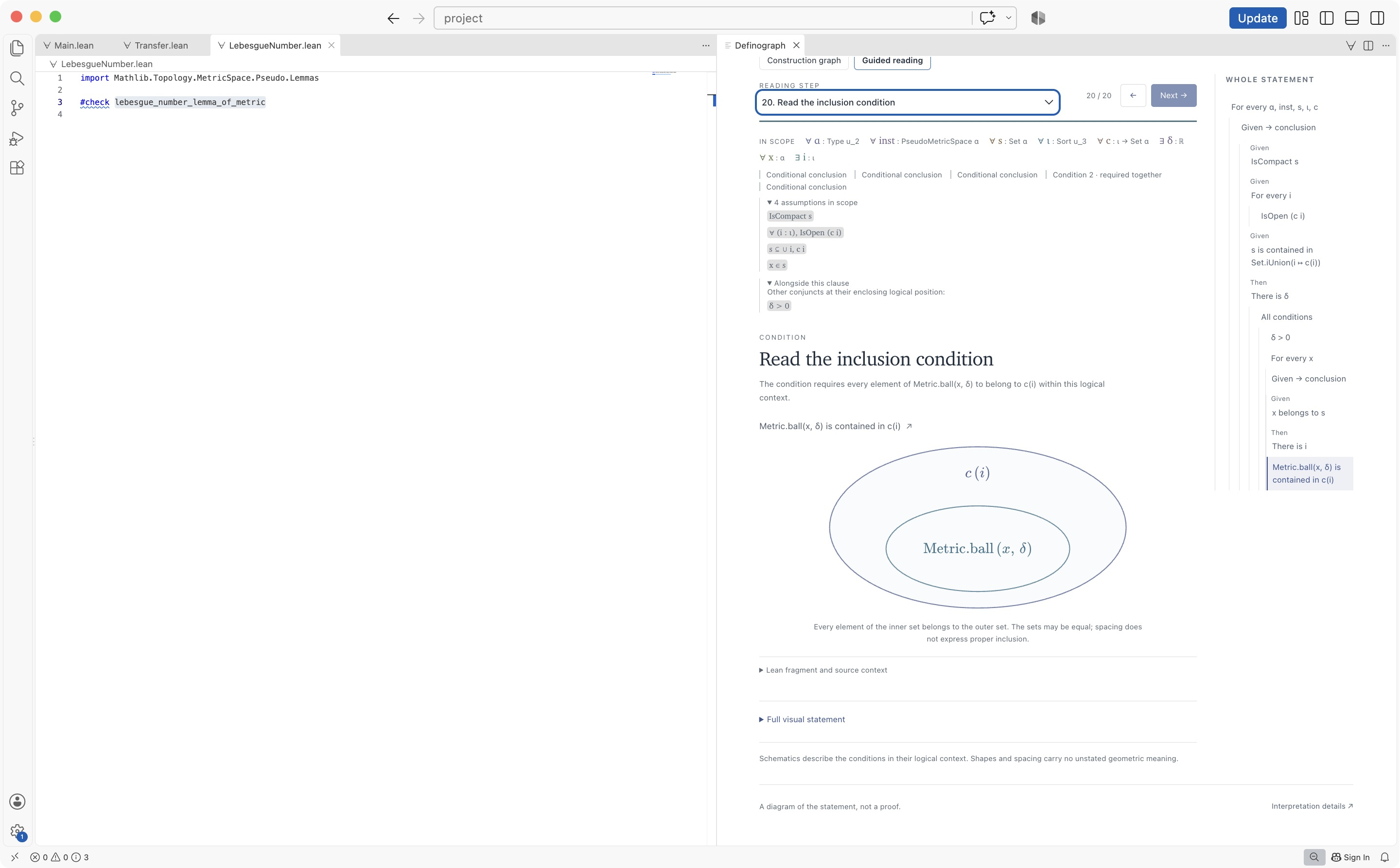
One complete reading

For the fixed compact set and open cover, there is one positive radius such that, for every center in the set, the entire ball of that radius lies in some cover member, whose index may depend on the center.

This describes the theorem’s statement. The view does not explain the proof or compute the radius and indices. If s is empty, there are no center-specific obligations; do not infer a selected point or a nonempty index family from the diagram.

Check your reading. Compare these conclusion forms for arbitrary sets and families, before using the theorem’s three hypotheses. Classify each change as equivalent, weaker, or stronger than the original conclusion:

Choose a new positive radius after each center x ∈ s.
Choose one cover member before all centers and require it to contain every ball.
Remove the restriction x ∈ s.

Answer: the changed statements

The first weakens the requirement: it loses the uniform radius. The second strengthens it by demanding one member for every center; the theorem does not guarantee this. The third also strengthens it, extending the requirement to arbitrary centers in the space. These conclusion forms are not equivalent in general, and a weaker statement should not simply be labelled false.

Try the same reading on a different statement

In pseudometric spaces, Metric.uniformContinuousOn_iff states the equivalence below for a function f : α → β and a set s : Set α. This is a separate reading exercise.

UniformContinuousOn f s ↔
  ∀ ε > 0, ∃ δ > 0, ∀ x ∈ s, ∀ y ∈ s,
    dist x y < δ → dist (f x) (f y) < ε

Does the theorem assert that this particular f is uniformly continuous? What may δ depend on? Are both points restricted to s?

Answer: follow the equivalence and the quantifiers

The theorem equates two conditions; it does not establish either one for an arbitrary f. For each positive ε, the right-hand side requires one positive δ that works for all later x,y ∈ s. The radius may depend on ε and the fixed data, but not on those later points.

Both points must lie in s, and dist x y < δ is an antecedent of the distance conclusion. Reading ↔ as only one implication would lose the converse.

The epsilon–delta expression comes from a proved equivalence theorem. It is not the definition body of UniformContinuousOn.

For more practice, use Lesson 1: the order of choices. Lesson 4 explains definition inspection, and Lesson 5 explains source checks in the editor.